In this lesson we will extend the SIR model to include demographic processes. In particular, we will include births and deaths from natural causes.
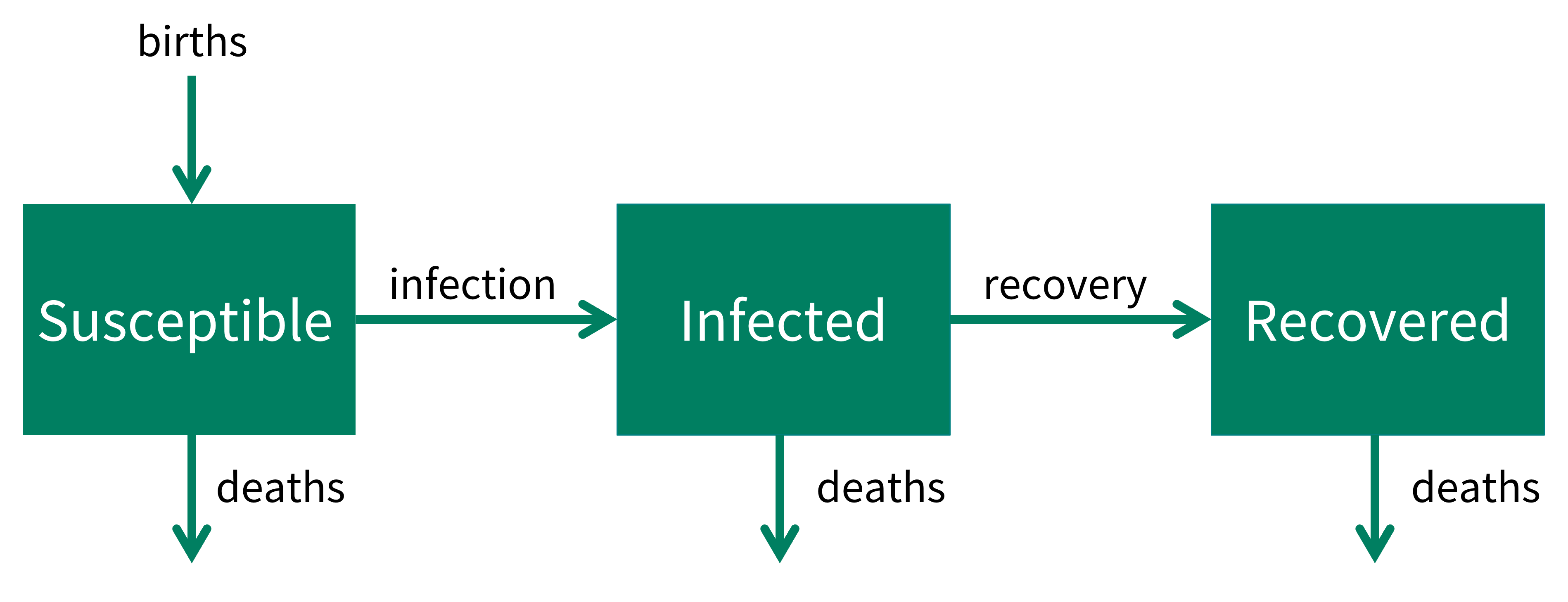
We assume all individuals, \(S\), \(I\) or \(R\) can give birth and all individuals are born susceptible. We assume deaths occur from natural causes, therefore deaths will occur at the same rate in each compartment. Our model assumptions are represented in the flow diagram below.
Notice that we now have arrows which do not always connect to other compartments, such as the deaths. This represents that once an individual dies, they do not move to another compartment.
We write down the our assumptions using words, \[
\begin{aligned}
\mbox{susceptible population rate of change} & = \mbox{births} - \mbox{infections} - \mbox{deaths} \\
\mbox{infected population rate of change} &= + \mbox{infections} - \mbox{recoveries} - \mbox{deaths}\\
\mbox{recovered population rate of change} &= + \mbox{recoveries} -\mbox{deaths}
\end{aligned}
\] We only have births entering the susceptible population, and we have deaths leaving the susceptible, infected and recovered population.
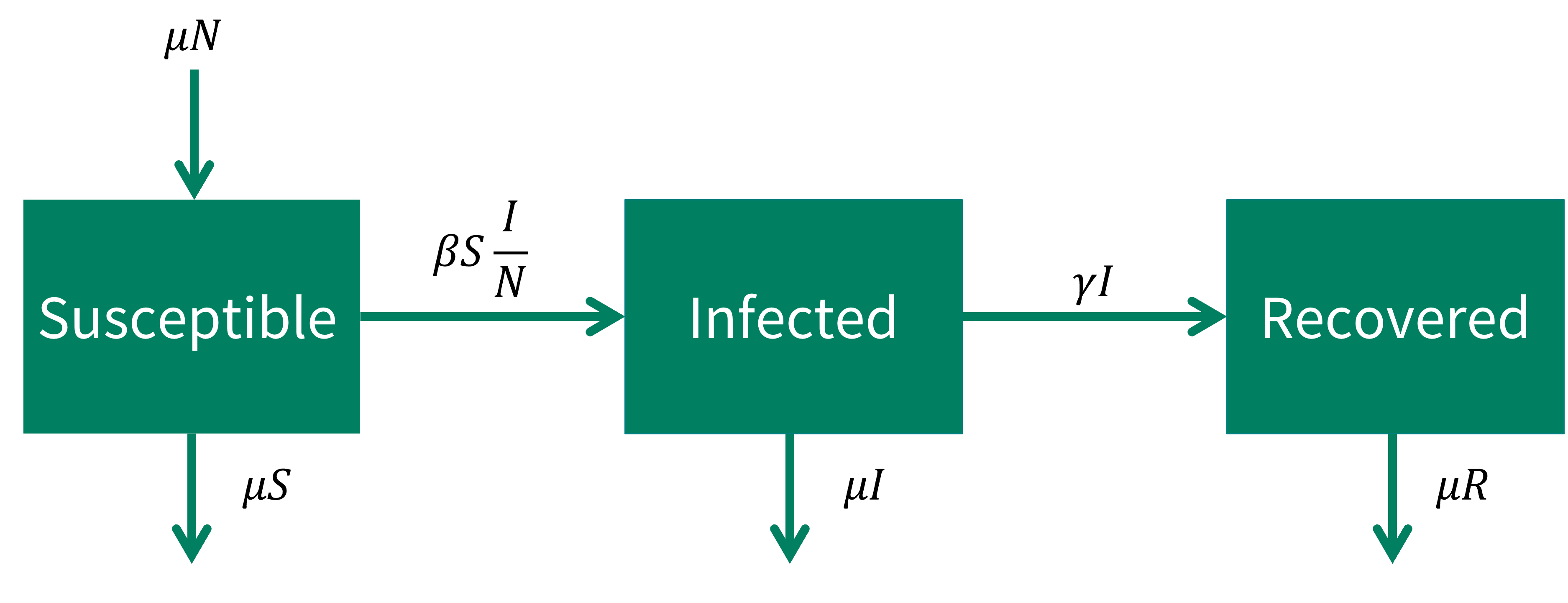
Given we assume all individuals are born susceptible, we have flows from each of \(S\), \(I\) and \(R\) back into \(S\). If we assume individuals are born at a per capita rate \(\mu\). Then the rate of new individuals born is \(\mu N\).
Individuals who die will leave the class but also leave the system entirely. We assume that births and deaths are equal, hence we also have a per capita death rate of \(\mu\). As death is from natural causes only, individuals die at the same rate from each class.
Our system of ODEs can be written as:
\[
\begin{aligned}
\frac{dS}{dt} & = \mu N- \beta S I/N - \mu S\\
\frac{dI}{dt} &= \beta S I/N - \gamma I - \mu I \\
\frac{dR}{dt} &=\gamma I - \mu R\\
\end{aligned}
\]
What will the solution to this system of ODEs look like?
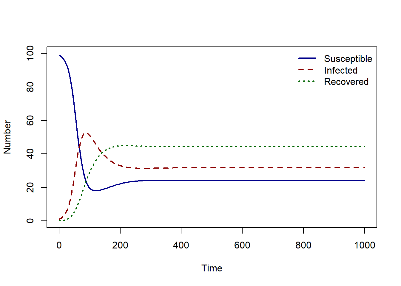
SIR_demography_model <-function(time, state_var, pars) {# Extract state variables S <- state_var["S"] I <- state_var["I"] R <- state_var["R"] N <- S + I + R# Extract model parameters beta <- pars["beta"] gamma <- pars["gamma"] mu <- pars["mu"]# The differential equations dS <- mu * N - beta * S * I / N - mu * S dI <- beta * S * I / N - gamma * I - mu * I dR <- gamma * I - mu * R# Return the equations as a list sol <-list(c(dS, dI, dR))return(sol)}# What are our parameter values?pars <-c(beta =0.1, gamma =0.014, mu =0.01)# Define time to solve equationstimes <-seq(from =0, to =1000, by =1)# What are the initial values (or conditions) of the state variables?state_var <-c(S =99, I =1, R =0)# Solve the Susceptible Infected equations over the vector of times , time# with initial conditionssolution <-as.data.frame(ode(y = state_var, times = times,func = SIR_demography_model, parms = pars,method = rk4))plot(solution$time, solution$S, col ="darkblue", lwd =2,type ="l", ylim =c(0, 100), ylab ="Number", xlab ="Time")lines(solution$time, solution$I, col ="darkred", lwd =2, lty =2)lines(solution$time, solution$R, col ="darkgreen", lwd =2, lty =3)legend("topright", c("Susceptible", "Infected", "Recovered"),col =c("darkblue", "darkred", "darkgreen"), lwd =2, lty =c(1, 2, 3),bty ="n")
We see there is an epidemic peak followed by an endemic state. In the SIR model with no births and deaths, we saw an epidemic peak which eventually died out. In the SIR model with births and deaths, new susceptible individuals are constantly being added to our population through birth. This addition of new susceptible results in infection becoming endemic.
Equilibrium states
An ODE system is at equilibrium when the rate of change of all variables is 0. i.e. \(\frac{dS}{dt}=0\), \(\frac{dI}{dt}=0\) and \(\frac{dR}{dt}=0\).
By setting the ODE equations to 0, in some cases we can find the analytical expression for the equilibrium state. We will denote the expressions for the equilibrium as \(S^*\), \(I^*\) and \(R^*\). We can use these expressions to find the value of the number of individuals infected at the endemic equilibrium.
For the SIR model with demography, there are two equilibrium states, either \(\frac{dS}{dt}=\frac{dI}{dt}=\frac{dR}{dt}=0\) because there is no infection or because infection is endemic. In the infection free equilibrium the values of the number of individuals in the \(S\), \(I\) and \(R\) class are: \[
\begin{aligned}
S^* &= N\\
I^* &= 0 \\
R^*&= 0
\end{aligned}
\]
And for the endemic equilibrium, \[
\begin{aligned}
S^* &= N\frac{1}{R_0} \\
I^* &= N(R_0 - 1)\frac{\mu}{\beta} \\
R^* &= N(R_0 - 1)\frac{\gamma}{\beta}
\end{aligned}
\]
where \(R_0 = \beta/(\gamma+\mu)\).
Using these equations and our parameter values, we can calculate the number of individuals in each disease state at equilibrium.
pars <-c(beta =0.1, gamma =0.014, mu =0.01)beta <- pars[["beta"]]gamma <- pars[["gamma"]]mu <- pars[["mu"]]R0 <- beta / (gamma + mu)N <-100S_star <- N * (1/ R0)I_star <- N * (R0 -1) * (mu / beta)R_star <- N * (R0 -1) * (gamma / beta)round(c(S_star, I_star, R_star), 4)
[1] 24.0000 31.6667 44.3333
We have found the value of the endemic prevalence without having to find the numerical solution.
However, this is a simple example and you may not always have an analytical expression of the equilibrium state, in this case, how can we find the endemic prevalence?
We can look at our numerical solution after the the epidemic peak. The R function tail will give us the last 6 rows of the solution data.frame.
tail(solution)
     time  S        I        R
996   995 24 31.66667 44.33333
997   996 24 31.66667 44.33333
998   997 24 31.66667 44.33333
999   998 24 31.66667 44.33333
1000  999 24 31.66667 44.33333
1001 1000 24 31.66667 44.33333
The values of our numerical solution are close to the analytical solution but not exact. We could try finding the solution for a longer time period, but we don’t know how long do we have to run our model to find endemic equilibrium.
We can use the R function runsteady()in the R package rootSolve to find a numerical approximation to the equilibrium state. This function takes the inputs of the value of the initial state variables, the R function for the ODE equations and the parameters.
Then we can extract the value of the equilibrium estimate y.
The numbers are now much more similar (to 4 decimal places). This is still an approximation to the true analytical solution, so we do not expect the answers to be identical.
Importance of demographic processes
We have shown that including births and deaths in an SIR model framework results in endemic infection. We have also shown that the birth and death rate \(\mu\) are in the expression for \(R_0\) and the endemic equilibrium.
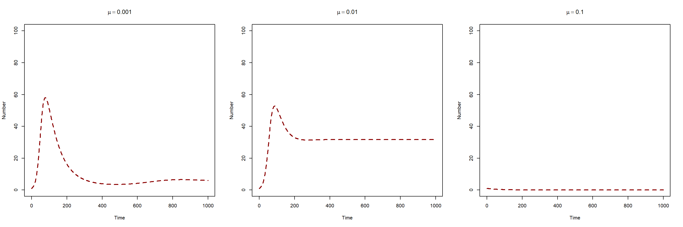
Let’s investigate the importance of including demographic processes by looking at the predicted epidemic for different values of \(\mu\).
When \(\mu\) is low in value, the infection spreads through the population so quickly that few births and deaths have occurred in that time-scale.
When \(\mu\) is higher in value (\(\mu = 0.01\)), the time-scale of infection is impacted by births, and so endemic infection occurs.
Finally, when \(\mu = 0.1\), the time-scale of infection is slow compared to births and deaths, and so the infection does not take off after the introduction of one infected individual.
If infection spreads quickly compared to the time-scale births and deaths, then demographic processes do not influence the infection dynamics. However, if infection spread is slow, then demographic processes may influence the level of endemic infection and if infection takes off at all.
The table below shows the values for \(R_0\) and the endemic equilibrium (\(I^*\)) for the three values of \(\mu\).
\(\mu\)
\(R_0\)
\(I^*\)
0.001
6.7
5.67
0.01
4.2
31.67
0.1
0.9
0
When \(\mu = 0.1\), \(R_0<1\) and so infection does not take off.
When \(R_0>1\), the highest \(R_0\) does not lead to the highest endemic equilibrium. This is important to note, \(R_0\) can tell you about likelihood of infection to take off, but the endemic equilibrium tells you about long term dynamics.
In summary, including births and deaths is a more realistic model of reality, and allows for the possibility of endemic infection. There are many extensions you can add to demographic processes in ODE models, including:
disease induced mortality
immunity at birth
infection at birth
control measures, such as vaccination at birth.
Exercise
How many compartments are in the SIR model with demography?
How many parameters are in the SIR model with demography (not including total population size \(N\))?
What are the numeric values of the endemic equilibrium state of the SIR model with demography and frequency dependent transmission with \(\beta=0.5\), \(\gamma =0.1\), \(\mu =0.05\) and \(N=200\)?
Solution
3 compartments : susceptible, infected and recovered.
There are three parameters, the transmission route \(\beta\), the recovery rate \(\gamma\) and the birth/death rate \(\mu\).
pars <-c(beta =0.5, gamma =1/10, mu =1/20)beta <- pars[["beta"]]gamma <- pars[["gamma"]]mu <- pars[["mu"]]R0 <- beta / (gamma + mu)N <-200S_star <- N * (1/ R0)I_star <- N * (R0 -1) * (mu / beta)R_star <- N * (R0 -1) * (gamma / beta)c(S_star, I_star, R_star)