SIRS_demography_model <- function(time, state_var, pars) {
  # Extract state variables
  S <- state_var["S"]
  I <- state_var["I"]
  R <- state_var["Z"]
  N <- S + I + R
  # Extract model parameters
  beta <- pars["beta"]
  gamma <- pars["gamma"]
  mu <- pars["mu"]
  # The differential equations
  dS <- mu * N + omega * R - beta * S * I / N - mu * S
  dI <- beta * S * I / N - gamma * I - mu * I
  dR <- gamma * I - mu * R - omega * R
  # Return the equations as a list
  sol <- list(c(dS, dI, dR))
  return(sol)
}

# What are our parameter values?
pars <- c(omega = 0.01, beta = 0.6, gama = 0.14, mu = 0.01)

# Define time to solve equations
times <- seq(from = 0, to = 250, by = 1)

# What are the initial values (or conditions) of the state variables?
state_var <- c(S = 99, I = 1, R = 0)

# Solve the Susceptible Infected equations over the vector of times , time
# with initial conditions
solution <- as.data.frame(ode(y = state_var, times = times,
                              func = SIRS_demography_model, parms = pars,
                              method = rk4))

plot(solution$time, solution$S, col = "darkblue", lwd = 2,
     type = "l", ylim = c(0, 100), ylab = "Number", xlab = "Time")
lines(solution$time, solution$I, col = "darkred", lwd = 2, lty = 2)
lines(solution$time, solution$R, col = "darkgreen", lwd = 2, lty = 3)
legend("topright", c("Susceptible", "Infected", "Recovered"),
       col = c("darkblue", "darkred", "darkgreen"),
lwd = 2, lty = c(1, 2, 3), bty = "n")Test your understanding
So far, we have learnt how to translate assumptions about how an infection spreads into ODE models. As well as formulating your own models, you may also be given model equations which you need to understand.
We have been given the following equations, let’s try to figure out assumptions this model includes using only the equations.
\[ \begin{aligned} \frac{dS}{dt} & = \mu N + \omega R - \beta S I/N - \mu S\\ \frac{dI}{dt} &= \beta S I/N - \gamma I - \mu I \\ \frac{dR}{dt} &=\gamma I - \mu R - \omega R\\ \end{aligned} \] By writing out the model equations in words, drawing a flow diagram, or both, can you infer what the model assumptions are?
Solution
There are three equations representing the rate of change in compartments \(S\), \(I\) and \(R\). The processes are formulated similarly to what we have seen before, but with the addition of one process described by some removal from \(R\) that moves to \(S\) at rate \(\omega R\).
We can write out the model equations in words, and refer to our additional process as ‘?’.
\[ \begin{aligned} \mbox{susceptible population rate of change} & = \mbox{births} + \mbox{?} - \mbox{infections} - \mbox{deaths} \\ \mbox{infected population rate of change} &= + \mbox{infections} - \mbox{recoveries} - \mbox{deaths}\\ \mbox{recovered population rate of change} &= + \mbox{recoveries} -\mbox{deaths} -\mbox{?} \end{aligned} \]
In flow diagram form this is, 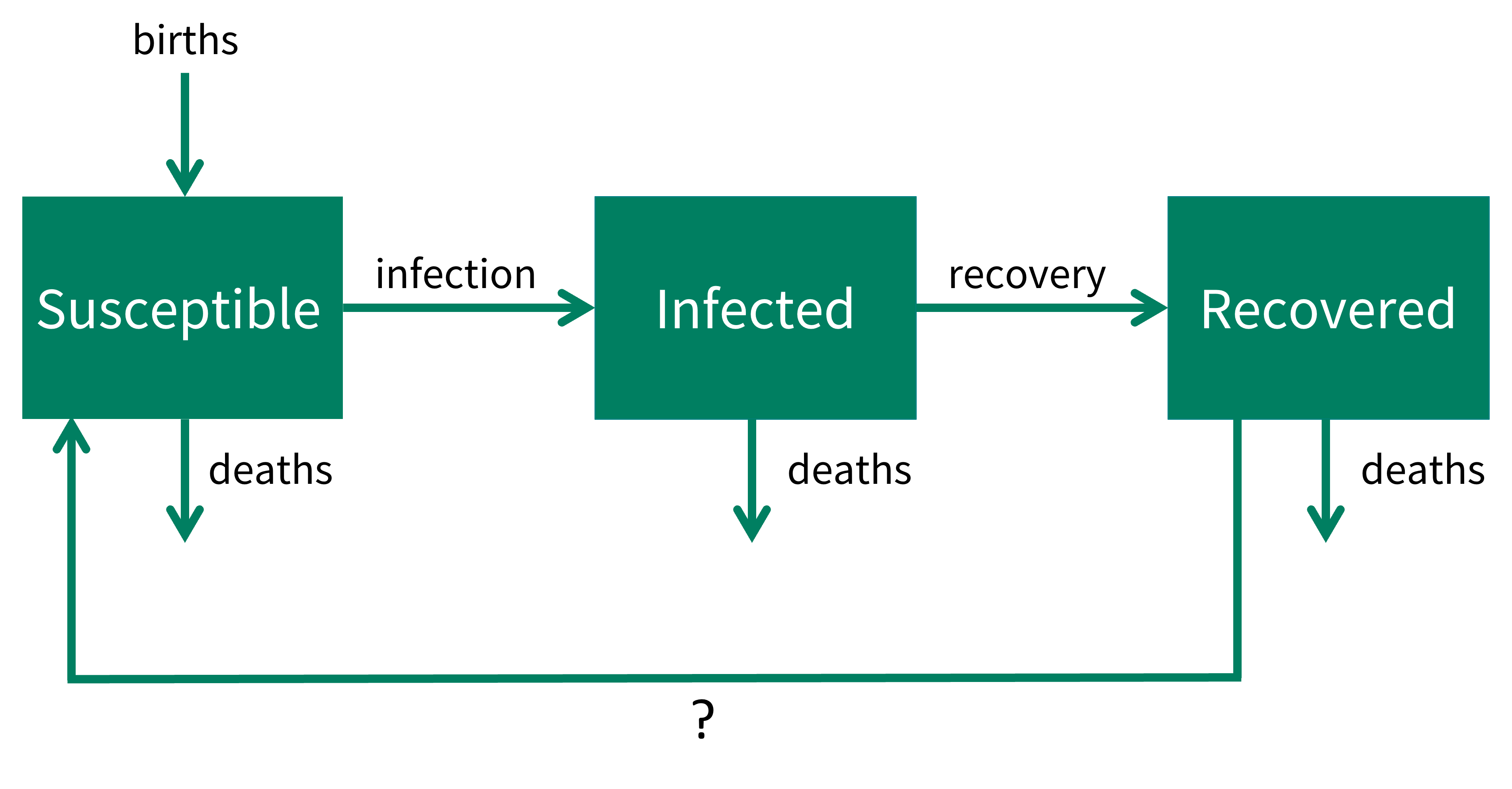
What biological process would result in individuals leaving the recovered class and moving to the susceptible class?
- loss of immunity

The model equations represent a Susceptible - Infected - Recovered - Susceptible (SIRS) model. In this model, individuals can recover from infection, but also lose their immunity after a period of time - and therefore become susceptible again.
Understanding code
We have also been given the following R code to find the numerical solution, but when we try to run the code, it doesn’t work. Can you fix the code and use the output to answer the questions in the next quiz?
Solution
The errors in the code were :
- within the model function, we need to extract
R <- state_var["R"]notR <- state_var["Z"]. This looks like a copy and paste mistake from a previous model. - within the model function, we need to extract
omegafrom the list of parameters. This line of code was missing, we add the lineomega <- pars["omega"]to the model code. - The name of the parameter \(\gamma\) did not match in the the parameter vector
parsand the model function. It was spelledgamainpars. We change this isgamma.
The fixed code is :
SIRS_demography_model <- function(time, state_var, pars) {
  # Extract state variables
  S <- state_var["S"]
  I <- state_var["I"]
  R <- state_var["R"]
  N <- S + I + R
  # Extract model parameters
  omega <- pars["omega"]
  beta <- pars["beta"]
  gamma <- pars["gamma"]
  mu <- pars["mu"]
  # The differential equations
  dS <- mu * N + omega * R - beta * S * I / N - mu * S
  dI <- beta * S * I / N - gamma * I - mu * I
  dR <- gamma * I - mu * R - omega * R
  # Return the equations as a list
  sol <- list(c(dS, dI, dR))
  return(sol)
}

# What are our parameter values?
pars <- c(omega = 0.01, beta = 0.6, gamma = 0.14, mu = 0.01)

# Define time to solve equations
times <- seq(from = 0, to = 250, by = 1)

# What are the initial values (or conditions) of the state variables?
state_var <- c(S = 99, I = 1, R = 0)

# Solve the Susceptible Infected equations over the vector of times , time
# with initial conditions
solution <- as.data.frame(ode(y = state_var, times = times,
                              func = SIRS_demography_model, parms = pars,
                              method = rk4))

plot(solution$time, solution$S, col = "darkblue", lwd = 2,
     type = "l", ylim = c(0, 100), ylab = "Number", xlab = "Time")
lines(solution$time, solution$I, col = "darkred", lwd = 2, lty = 2)
lines(solution$time, solution$R, col = "darkgreen", lwd = 2, lty = 3)
legend("topright", c("Susceptible", "Infected", "Recovered"),
       col = c("darkblue", "darkred", "darkgreen"), lwd = 2, lty = c(1, 2, 3),
       bty = "n")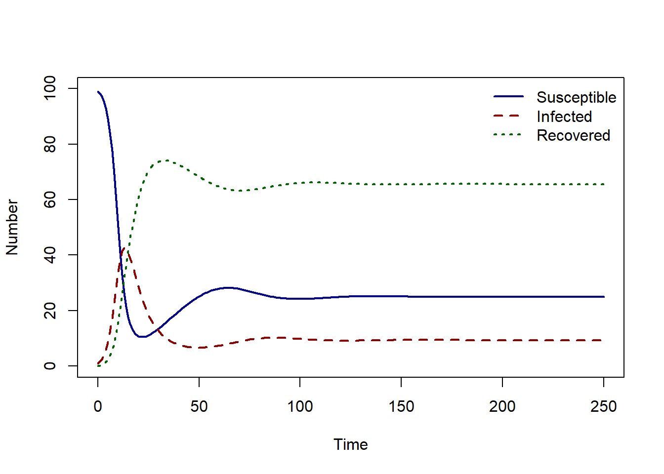
In the SIRS model solution, after the epidemic peak, the recovered individuals lose their immunity and become susceptible again, resulting in a secondary peak followed by endemic infection in the population.
We can find the endemic equilibrium values using runsteady.
equilibrium_state <- runsteady(y = state_var,
                               func = SIRS_demography_model, parms = pars)
print(round(equilibrium_state$y, 2))
S I R
25.00 9.37 65.63
Exercise
If you increase the rate of loss of immunity, what is the effect on the number of infectious individuals at the endemic equilibrium?
Solution
pars <- c(omega = 0.05, beta = 0.6, gamma = 0.14, mu = 0.01)

equilibrium_state <- runsteady(y = state_var,
                               func = SIRS_demography_model, parms = pars)
print(round(equilibrium_state$y, 2))
S I R
25.0 22.5 52.5 The number of infectious individuals at endemic equilibrium increases.