The Susceptible - Infected model
As modellers, we specify the rate of change of our variable of interest based on our assumptions about biological processes. The key to understanding epidemic models is to understand the assumptions being made about infection spread, and the impact of these assumptions on the predicted dynamics over time.
The Susceptible - Infected model
The first model we will introduce is the Susceptible – Infected or SI model. In this model, individuals are in one of two disease states, susceptible or infected (and infectious). We refer to these disease states as different ‘compartments’.
The schematic below represents our model in the form of a flow diagram. There are two compartments: ‘S’ for susceptible and ‘I’ for infected, and there is one process whereby individuals can move from ‘S’ to ‘I’, infection:

To predict the flow between the two compartments, we will use ordinary differential equations (ODEs). Here we are interested in modelling the rate of change of the number of individuals in each compartment with respect to time.
We will write an ODE for each compartment. Therefore we will have two equations. We have one process whereby individuals leave the ‘S’ class and those same individuals are added to the ‘I’ class:
\[ \begin{aligned} \mbox{susceptible population rate of change} & = - \mbox{infections} \\ \mbox{infected population rate of change} &= + \mbox{infections} \end{aligned} \]
We denote the number of susceptible \(S\) and the number of infected individuals \(I\). We are interested in the rate of population change of these variable \(S\) and \(I\) over time, which we will denote \(t\).
The susceptible population rate of change with respect to time is written as \(\frac{dS}{dt}\) (similarly the infected population rate of change is \(\frac{dI}{dt}\)).
In this model, the population rate of change is defined by only one process : infection. Next we must formulate the rate of new infections per time unit as a function of:
- the number of susceptible individuals (\(S\))
- the probability that a susceptible contacts an infected individual (\(p\))
- the rate of contact between susceptible and infected individuals (\(c\))
- probability of successful transmission given contact (\(\nu\))
Our infection process from \(S\) to \(I\) can be written as the product of these terms:
\[ c \nu S p \] the probability that a susceptible individual contacts an infected individual is equal to the current prevalence, therefore, we can use \(p = I/N\).
The product of the rate of contact and the probability of successful transmission given contact gives the overall transmission rate, which we denote \(\beta\). Therefore, \(\beta = c \nu\).
Our infection process can be written as:
\[ \beta S I \] The individuals leave \(S\) at the same rate as they move to \(I\). Therefore we write the same terms in both \(dS/dt\) and \(dI/dt\) but with different signs to represent the loss of individuals from the susceptible class and the gain in individuals to the infected class.
\[ \begin{aligned} \frac{dS}{dt} & = - \beta S I \\ \frac{dI}{dt} &= \beta S I \end{aligned} \]
Now we will use these equations to find the predicted proportions of individuals in each class. Recall that the to find the solution to a differential equation, we integrate.
Notation: we have state variables \(S\) and \(I\). We assume we know the numbers of individuals in \(S\) and \(I\) at time 0. If we assume there is one infected individual in a population of 100 people, we denote the initial state at time 0 as \(S(0) = 99\) and \(I(0) = 1\).
We have just one parameter, \(\beta\).
Later in the course, we will learn how to perform numerical integration in R, for now we will focus on understanding what output we might expect given equations.
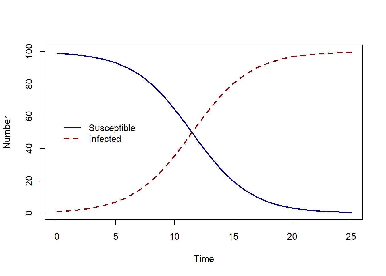
In this case, what do you think the predicted numbers of susceptible individual and infected individual over time will look like?
The SI model continued
The plot below shows the predicted numbers over time. We see that the number of infected individuals increases over time. As the outbreak progresses, more susceptible individuals become infected.
Eventually all individuals become infected. This is because in our system of ODEs there is only one process and only one direction to that process : susceptible individuals becoming infected.
One behaviour we can predict using the equation, is the speed at which the infection spreads. To explore this, we can look at the predicted numbers for different transmission rates \(\beta = 0.4\), \(\beta = 0.1\) and \(\beta = 1.5\).
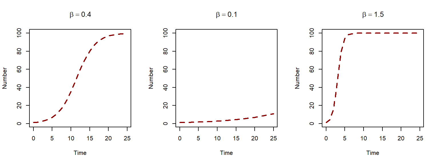
The higher the value of \(\beta\) the quicker the infection spreads. In the next lesson, we will look at extending our model to include the possibility of recovering from infection.
Exercise
- How many compartments are in the SI model?
- How many parameters are in the SI model (not including total population size \(N\))?
Solution
- There are two compartments : susceptible and infected
- There is one parameter, the transmission route \(\beta\).