data("women")
plot(women$weight, women$height)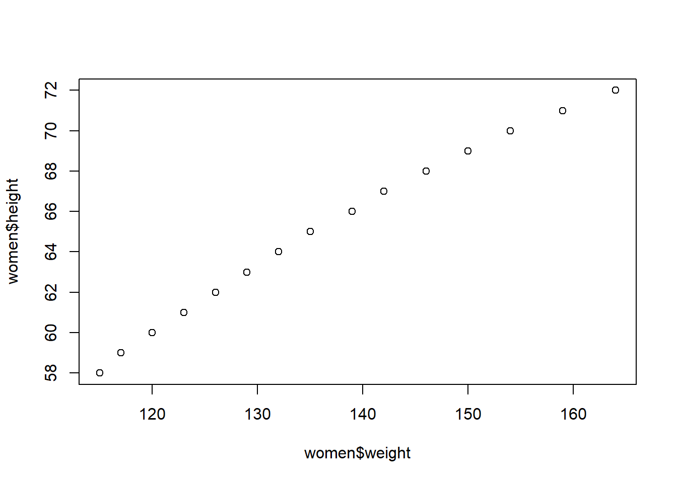
R can be used for data analysis and manipulating data. In both of these cases, we want to be able to plot our data.
The code below loads in the data set women and makes a basic scatter plot of height against weight. Copy and paste this R code into your R script then run the lines. The plot below will appear in your Files / Plots / Packages / Help panel.
data("women")
plot(women$weight, women$height)
At the moment, our plot isn’t easy to read, the axis labels are not clear. We can improve it by changing our axis labels using xlab for changing the x axis label and ylab for changing the y axis label.
plot(women$weight, women$height,
     xlab = "Weight (lbs)", ylab = "Height (in)")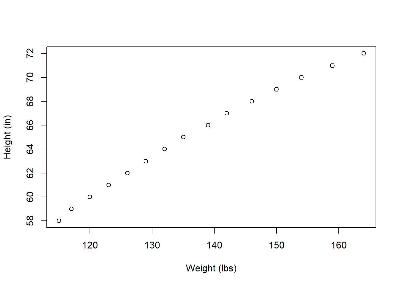
Let’s also add a main title, to do this we use the argument main.
plot(women$weight, women$height,
     xlab = "Weight (lbs)", ylab = "Height (in)",
     main = "Plot of weight against height")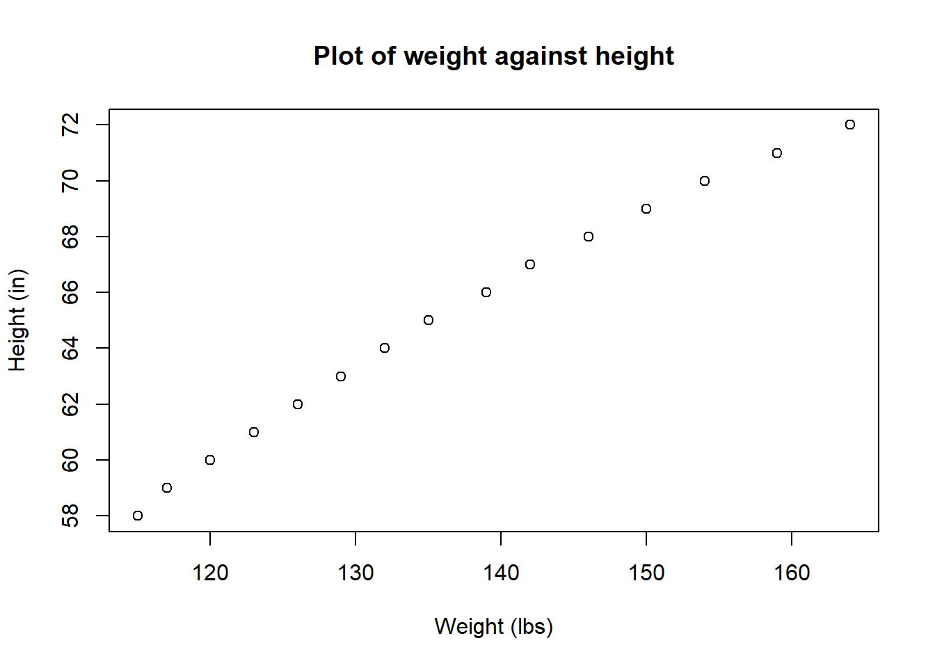
We can change the colour of the points using col = "blue" and change the shape of the points using pch.
plot(women$weight, women$height,
     xlab = "Weight (lbs)", ylab = "Height (in)",
     main = "Plot of weight against height",
     pch = 19, col = "blue")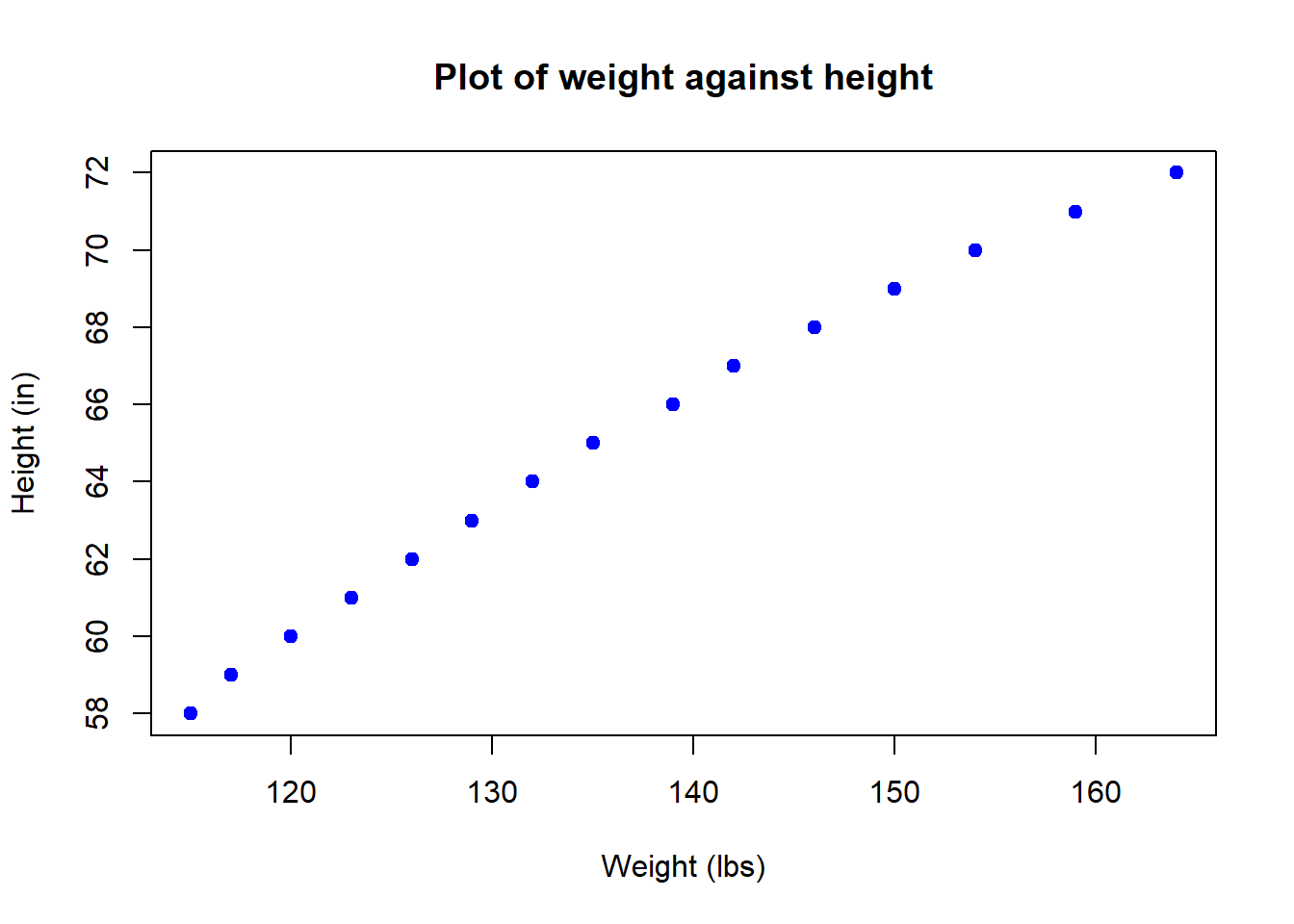
To save our plot, we can click on Export (just above the plot) and either save as Image or PDF. Select as Image. You change the name of the file in the ‘File Name:’ box.
If you selected a folder to be your working directory, then the plot should appear in that folder. To check what your current working director is type getwd() into the console.
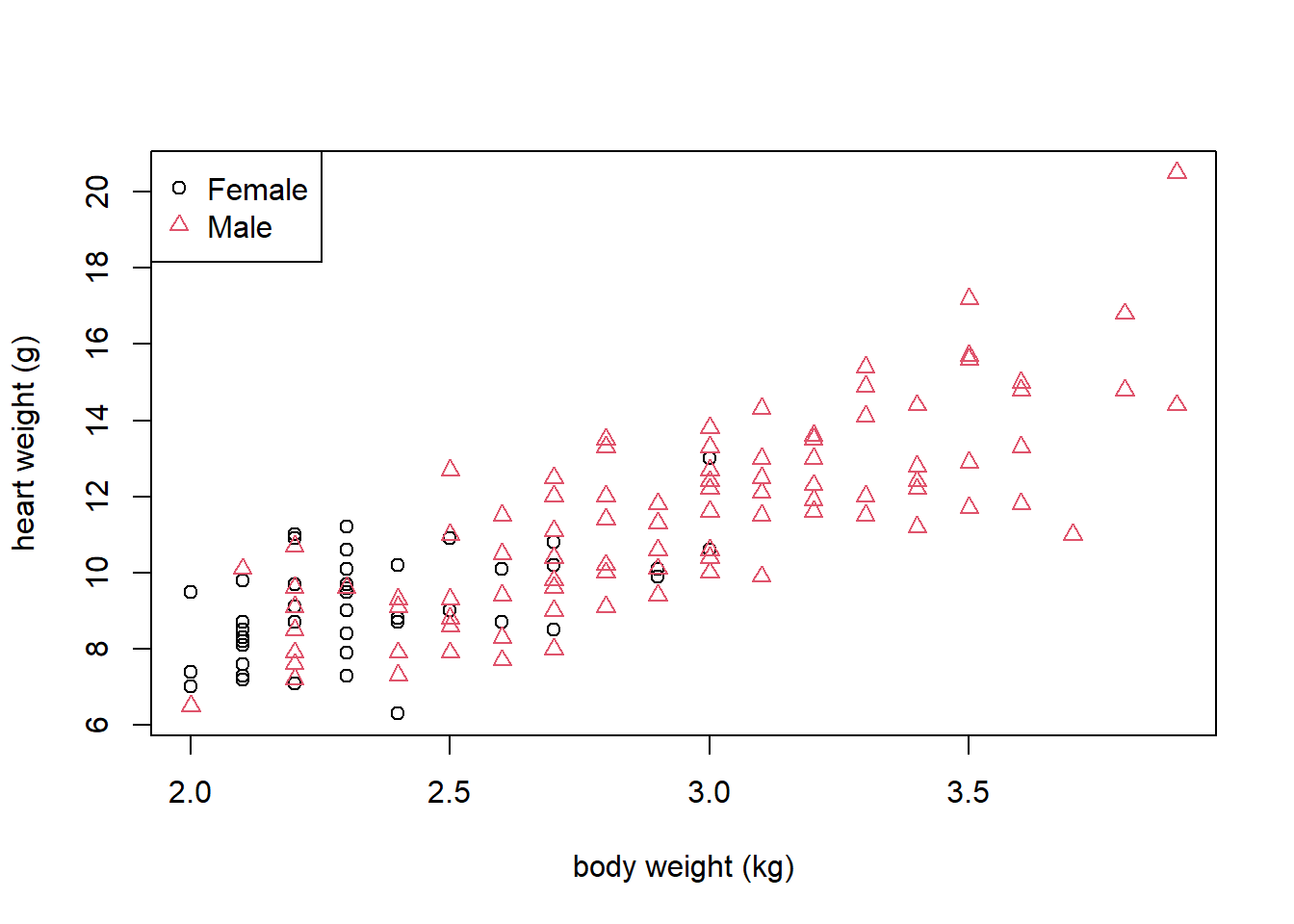
The code below loads the data set cats from the MASS package and makes a basic scatter plot of body weight against heart weight.
library(MASS)
plot(cats$Bwt, cats$Hwt)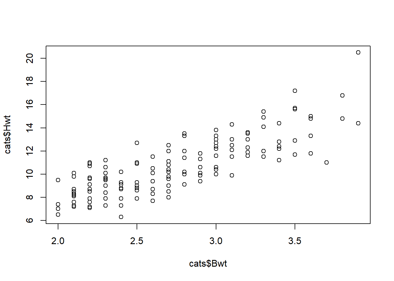
Download and install the package MASS then extend the code above, to recreate the plot below (hint : you can specify col and pch as one number or a vector of numbers).

library(MASS)
plot(cats$Bwt, cats$Hwt, pch = as.numeric(cats$Sex),
     xlab = "body weight (kg)", ylab = "heart weight (g)",
     col = as.numeric(cats$Sex))
legend("topleft", legend = c("Female", "Male"), pch = c(1, 2), col = c(1, 2))